 c
c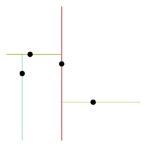 d
d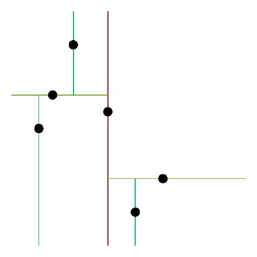
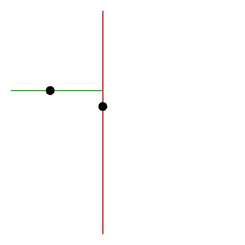
This division process induces a binary tree structure: The first point becomes the root, and each point falling into the left half-plane is inserted into the left subtree, and each point falling into the right half-plane is inserted into the right subtree. For points that divide regions horizontally, the points in the upper half-plane are inserted into the left subtree whereas points in the lower half-plane are inserted into the right subtree. Thus, nodes at even levels in the tree divide the set of points into left and right half-regions, and nodes at odd levels divide a region into upper and lower half-regions.
There are two obvious views of this algorithm: a view of the partitioning of the plane, and a view of the binary tree that is induced. The 3D view shown belows merges and unites these two views.
The points in the plane are drawn as circles in the xy plane, and the partitionings caused by them are drawn as transparent walls extended in the z dimension. On top of each wall and above each point is a sphere, representing the corresponding node in the 2-d tree. Therefore, the height (as well as color) of each wall reflects the node's level in the tree. The tree edges are represented as lines connecting related nodes.
When viewed from the top and with the tree edges hidden, as in Figs. a, c, and e, we see the traditional view of the partitioning of the plane. Exposing the tree edges would show the 2-d tree in a representation that a graph-theorist would be comfortable with: as a connected, acyclic graph. However, when viewed from the side (and with the walls mostly transluscent), as in Figs. b, d, and f, we see a tree more familiar to the computer scientist: each node is below its parent.
Figs. a and b show the state of the algorithm after it has processed the first two points. Figs. c and d show the state after the algorithm has processed the third and fourth points, and Figs. e and f, after the algorithm has processed the fifth and sixth points. Finally, Fig. g shows the state of the algorithm after all points have been processed, with opaque partitioning walls. Notice how the 3D view merges the traditional plane-partitioning view and the induced 2-d tree view.
a
c
d
b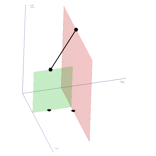 d
d f
f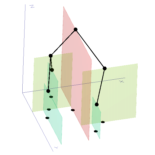
g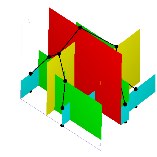
It is disconcerting to see edges of the tree overlapping. (Moreover, the left and right children are not necessarily drawn to the left and right of their parent!) Fortunately, when the tree is rotated in real-time about the z axis, it appears to have depth. The real-time animation provides the viewer with the visual clues needed to understand the overlaps.