Linear model
From Wikipedia, the free encyclopedia
In statistics, given a (random) sample  the most general form of linear model is formulated as

where  may be nonlinear functions.
In matrix notation this model can be written as

where Y is an n × 1 column vector, X is an n × (p + 1) matrix, β is a (p + 1) × 1 vector of (unobservable) parameters, and ε is an n × 1 vector of errors, which are uncorrelated random variables each with expected value 0 and variance σ2. Note that depending on the context the sample can be seen as fixed (observable), or random.
Much of the theory of linear models is associated with inferring the values of the parameters β and σ2. Typically this is done using the method of maximum likelihood, which in the case of normal errors is equivalent to the method of least squares.
Contents |
[edit] Assumptions
[edit] Multivariate normal errors
Often one takes the components of the vector of errors to be independent and normally distributed, giving Y a multivariate normal distribution with mean Xβ and co-variance matrix σ2 I, where I is the identity matrix. Having observed the values of X and Y, the statistician must estimate β and σ2.
[edit] Rank of X
We usually assume that X is of full rank p, which allows us to invert the p × p matrix  . The essence of this assumption is that the parameters are not linearly dependent upon one another, which would make little sense in a linear model. This also ensures the model is identifiable.
[edit] Methods of inference
[edit] Maximum likelihood
[edit] β
The log-likelihood function (for εi independent and normally distributed) is

where  is the ith row of X. Differentiating with respect to βj, we get

so setting this set of p equations to zero and solving for β gives

Now, using the assumption that X has rank p, we can invert the matrix on the left hand side to give the maximum likelihood estimate for β:
 .
.
We can check that this is a maximum by looking at the Hessian matrix of the log-likelihood function.
[edit] σ2
By setting the right hand side of
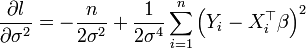
to zero and solving for σ2 we find that

[edit] Accuracy of maximum likelihood estimation
Since we have that Y follows a multivariate normal distribution with mean Xβ and co-variance matrix σ2 I, we can deduce the distribution of the MLE of β:

So this estimate is unbiased for β, and we can show that this variance achieves the Cramér-Rao bound.
A more complicated argument[1] shows that

since a chi-squared distribution with n − p degrees of freedom has mean n − p, this is only asymptotically unbiased.
[edit] Generalizations
[edit] Generalized least squares
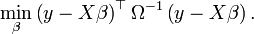
If, rather than taking the variance of ε to be σ2I, where I is the n×n identity matrix, one assumes the variance is σ2Ω, where Ω is a known matrix other than the identity matrix, then one estimates β by the method of "generalized least squares", in which, instead of minimizing the sum of squares of the residuals, one minimizes a different quadratic form in the residuals — the quadratic form being the one given by the matrix Ω−1:
This has the effect of "de-correlating" normal errors, and leads to the estimator

which is the best linear unbiased estimator for β. If all of the off-diagonal entries in the matrix Ω are 0, then one normally estimates β by the method of weighted least squares, with weights proportional to the reciprocals of the diagonal entries. The GLS estimator is also known as the Aitken estimator, after Alexander Aitken, the Professor in the University of Otago Statistics Department who pioneered it.[2]
[edit] Generalized linear models
Generalized linear models, for which rather than
- E(Y) = Xβ,
one has
- g(E(Y)) = Xβ,
where g is the "link function". The variance is also not restricted to being normal.
An example is the Poisson regression model, which states that
- Yi has a Poisson distribution with expected value eγ+δxi.
The link function is the natural logarithm function. Having observed xi and Yi for i = 1, ..., n, one can estimate γ and δ by the method of maximum likelihood.
[edit] References
- ^ A.C. Davidson Statistical Models. Cambridge University Press (2003).
- ^ Alexander Craig Aitken
[edit] See also
- ANOVA, or analysis of variance, is historically a precursor to the development of linear models. Here the model parameters themselves are not computed, but X column contributions and their significance are identified using the ratios of within-group variances to the error variance and applying the F test.
- Linear regression
- Robust regression

