Variance

From Wikipedia, the free encyclopedia

This article is about mathematics. For the administrative exception to land use regulations, see variance (land use).

In probability theory and statistics, the variance of a random variable, probability distribution, or sample is one measure of statistical dispersion, averaging the squared distance of its possible values from the expected value (mean). Whereas the mean is a way to describe the location of a distribution, the variance is a way to capture its scale or degree of being spread out. The unit of variance is the square of the unit of the original variable. The positive square root of the variance, called the standard deviation, has the same units as the original variable and can be easier to interpret for this reason.

The variance of a real-valued random variable is its second central moment, and it also happens to be its second cumulant. Just as some distributions do not have a mean, some do not have a variance. The mean exists whenever the variance exists, but not vice versa.

[edit] Definition

If random variable X has expected value (mean) μ = E(X), then the variance Var(X) of X is given by:

$\operatorname{Var}(X) = \operatorname{E}[ ( X - \mu ) ^ 2 ].\,$

This definition encompasses random variables that are discrete, continuous, or neither. Of all the points about which squared deviations could have been calculated, the mean produces the minimum value for the averaged sum of squared deviations.

The variance of random variable X is typically designated as Var(X), $\scriptstyle\sigma_X^2$ , or simply σ². If a distribution does not have an expected value, as is the case for the Cauchy distribution, it does not have a variance either. Many other distributions for which the expected value does exist do not have a finite variance because the relevant integral diverges. An example is a Pareto distribution whose Pareto index k satisfies 1 < k ≤ 2.

[edit] Continuous case

If the random variable X is continuous with probability density function p(x),

$\operatorname{Var}(X) =\int (x-\mu)^2 \, p(x) \, dx\,,$

where

$\mu = \int x \, p(x) \, dx\,,$

and where the integrals are definite integrals taken for x ranging over the range of X.

[edit] Discrete case

If the random variable X is discrete with probability mass function x₁ ↦ p₁, ..., x_n ↦ p_n,

$\sum_{i=1}^n p_i (x_i - \mu)^2\,.$

(Note: this variance should be divided by the sum of weights in the case of a discrete weighted variance.) That is, it is the expected value of the square of the deviation of X from its own mean. In plain language, it can be expressed as "The average of the square of the distance of each data point from the mean". It is thus the mean squared deviation.

[edit] Examples

[edit] Exponential distribution

The exponential distribution with parameter λ is a continuous distribution whose support is the semi-infinite interval [0,∞). Its probability density function is given by:

$f(x) = \lambda e^{-\lambda x},\,$

and it has expected value μ = λ⁻¹. Therefore the variance is equal to:

$\int_0^\infty f(x) (x - \mu)^2\,dx = \int_0^\infty \lambda e^{-\lambda x} (x - \lambda^{-1})^2\,dx = \lambda^{-2}.\,$

So for an exponentially distributed random variable σ² = μ².

[edit] Fair die

A six-sided fair die can be modelled with a discrete random variable with outcomes 1 through 6, each with equal probability ¹/₆. The expected value is (1+2+3+4+5+6)/6 = 3.5. Therefore the variance can be computed to be:

$\sum_{i=1}^6 \tfrac{1}{6} (i - 3.5)^2 = \tfrac{1}{6}\left((-2.5)^2{+}(-1.5)^2{+}(-0.5)^2{+}0.5^2{+}1.5^2{+}2.5^2\right) = \tfrac{1}{6} \cdot 17.50 = \tfrac{35}{12} \approx 2.92\,.$

[edit] Properties

Variance is non-negative because the squares are positive or zero. The variance of a constant random variable is zero, and the variance of a variable in a data set is 0 if and only if all entries have the same value.

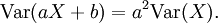
Variance is invariant with respect to changes in a location parameter. That is, if a constant is added to all values of the variable, the variance is unchanged. If all values are scaled by a constant, the variance is scaled by the square of that constant. These two properties can be expressed in the following formula:

$\operatorname{Var}(aX+b)=a^2\operatorname{Var}(X).$

The variance of a finite sum of uncorrelated random variables is equal to the sum of their variances. This stems from the identity:

$\operatorname{Var}(X+Y)=\operatorname{Var}(X)+\operatorname{Var}(Y)+2\operatorname{cov}(X,Y),$

and that for uncorrelated variables covariance is zero.

Suppose that the observations can be partitioned into subgroups according to some second variable. Then the variance of the total group is equal to the mean of the variances of the subgroups plus the variance of the means of the subgroups. This property is known as variance decomposition or the law of total variance and plays an important role in the analysis of variance. For example, suppose that a group consists of a subgroup of men and an equally large subgroup of women. Suppose that the men have a mean body length of 180 and that the variance of their lengths is 100. Suppose that the women have a mean length of 160 and that the variance of their lengths is 50. Then the mean of the variances is (100 + 50) / 2 = 75; the variance of the means is the variance of 180, 160 which is 100. Then, for the total group of men and women combined, the variance of the body lengths will be 75 + 100 = 175. Note that this uses N for the denominator instead of N - 1.
In a more general case, if the subgroups have unequal sizes, then they must be weighted proportionally to their size in the computations of the means and variances. The formula is also valid with more than two groups, and even if the grouping variable is continuous.[2]

This formula implies that the variance of the total group cannot be smaller than the mean of the variances of the subgroups. Note, however, that the total variance is not necessarily larger than the variances of the subgroups. In the above example, when the subgroups are analyzed separately, the variance is influenced only by the man-man differences and the woman-woman differences. If the two groups are combined, however, then the men-women differences enter into the variance also.
Many computational formulas for the variance are based on this equality: The variance is equal to the mean of the squares minus the square of the mean. For example, if we consider the numbers 1, 2, 3, 4 then the mean of the squares is (1 × 1 + 2 × 2 + 3 × 3 + 4 × 4) / 4 = 7.5. The mean is 2.5, so the square of the mean is 6.25. Therefore the variance is 7.5 − 6.25 = 1.25, which is indeed the same result obtained earlier with the definition formulas. Many pocket calculators use an algorithm that is based on this formula and that allows them to compute the variance while the data are entered, without storing all values in memory. The algorithm is to adjust only three variables when a new data value is entered: The number of data entered so far (n), the sum of the values so far (S), and the sum of the squared values so far (SS). For example, if the data are 1, 2, 3, 4, then after entering the first value, the algorithm would have n = 1, S = 1 and SS = 1. After entering the second value (2), it would have n = 2, S = 3 and SS = 5. When all data are entered, it would have n = 4, S = 10 and SS = 30. Next, the mean is computed as M = S / n, and finally the variance is computed as SS / n − M × M. In this example the outcome would be 30 / 4 - 2.5 × 2.5 = 7.5 − 6.25 = 1.25. If the unbiased sample estimate is to be computed, the outcome will be multiplied by n / (n − 1), which yields 1.667 in this example.

[edit] Properties, formal

[edit] Variance of the sum of uncorrelated variables (Bienaymé formula)

One reason for the use of the variance in preference to other measures of dispersion is that the variance of the sum (or the difference) of uncorrelated random variables is the sum of their variances:

$\operatorname{Var}\Big(\sum_{i=1}^n X_i\Big) = \sum_{i=1}^n \operatorname{Var}(X_i).$

This statement is called the Bienaymé formula.^[1] and was discovered in 1853. It is often made with the stronger condition that the variables are independent, but uncorrelatedness suffices. So if the variables have the same variance σ², then, since division by n is a linear transformation, this formula immediately implies that the variance of their mean is

$\operatorname{Var}(\overline{X}) = \operatorname{Var}\left(\frac{1}{n}\sum_{i=1}^n X_i\right) = \frac {1}{n^2} n \sigma^2 = \frac {\sigma^2} {n}.$

That is, the variance of the mean decreases with n. This fact is used in the definition of the standard error of the sample mean, which is used in the central limit theorem.

[edit] Variance of the sum of correlated variables

In general, if the variables are correlated, then the variance of their sum is the sum of their covariances:

$\operatorname{Var}\left(\sum_{i=1}^n X_i\right) = \sum_{i=1}^n \sum_{j=1}^n \operatorname{Cov}(X_i, X_j).$

(Note: This by definition includes the variance of each variable, since Cov(X,X)=Var(X).)

Here Cov is the covariance, which is zero for independent random variables (if it exists). The formula states that the variance of a sum is equal to the sum of all elements in the covariance matrix of the components. This formula is used in the theory of Cronbach's alpha in classical test theory.

So if the variables have equal variance σ² and the average correlation of distinct variables is ρ, then the variance of their mean is

$\operatorname{Var}(\overline{X}) = \frac {\sigma^2} {n} + \frac {n-1} {n} \rho \sigma^2.$

This implies that the variance of the mean increases with the average of the correlations. Moreover, if the variables have unit variance, for example if they are standardized, then this simplifies to

$\operatorname{Var}(\overline{X}) = \frac {1} {n} + \frac {n-1} {n} \rho.$

This formula is used in the Spearman-Brown prediction formula of classical test theory. This converges to ρ if n goes to infinity, provided that the average correlation remains constant or converges too. So for the variance of the mean of standardized variables with equal correlations or converging average correlation we have

$\lim_{n \to \infty} \operatorname{Var}(\overline{X}) = \rho.$

Therefore, the variance of the mean of a large number of standardized variables is approximately equal to their average correlation. This makes clear that the sample mean of correlated variables does generally not converge to the population mean, even though the Law of large numbers states that the sample mean will converge for independent variables.

[edit] Variance of a weighted sum of variables

Properties 6 and 8, along with this property from the covariance page: Cov(aX, bY) = ab Cov(X, Y) jointly imply that

$\operatorname{Var}(aX+bY) =a^2 \operatorname{Var}(X) + b^2 \operatorname{Var}(Y) + 2ab\, \operatorname{Cov}(X, Y).$

This implies that in a weighted sum of variables, the variable with the largest weight will have a disproportionally large weight in the variance of the total. For example, if X and Y are uncorrelated and the weight of X is two times the weight of Y, then the weight of the variance of X will be four times the weight of the variance of Y.

[edit] Decomposition of variance

The general formula for variance decomposition or the law of total variance is: If X and Y are two random variables and the variance of X exists, then

$\operatorname{Var}(X) = \operatorname{Var}(\operatorname{E}(X|Y))+ \operatorname{E}(\operatorname{Var}(X|Y)).$

Here, E(X|Y) is the conditional expectation of X given Y, and Var(X|Y) is the conditional variance of X given Y. (A more intuitive explanation is that given a particular value of Y, then X follows a distribution with mean E(X|Y) and variance Var(X|Y). The above formula tells how to find Var(X) based on the distributions of these two quantities when Y is allowed to vary.) This formula is often applied in analysis of variance, where the corresponding formula is

S S Total = S S Between + S S Within .

It is also used in linear regression analysis, where the corresponding formula is

S S Total = S S Regression + S S Residual .

This can also be derived from the additivity of variances (property 8), since the total (observed) score is the sum of the predicted score and the error score, where the latter two are uncorrelated.

[edit] Computational formula for variance

Main article: computational formula for the variance

The computational formula for the variance follows in a straightforward manner from the linearity of expected values and the above definition:

${}\operatorname{Var}(X)= \operatorname{E}(X^2 - 2\,X\,\operatorname{E}(X) + (\operatorname{E}(X))^2),$

${}=\operatorname{E}(X^2) - 2(\operatorname{E}(X))^2 + (\operatorname{E}(X))^2,$

${}=\operatorname{E}(X^2) - (\operatorname{E}(X))^2.$

This is often used to calculate the variance in practice, although it suffers from catastrophic cancellation if the two components of the equation are similar in magnitude.

[edit] Characteristic property

The second moment of a random variable attains the minimum value when taken around the first moment (i.e., mean) of the random variable, i.e. $\mathrm{argmin}_m\,\mathrm{E}((X - m)^2) = \mathrm{E}(X)\,$ . Conversely, if a continuous function $\varphi$ satisfies $\mathrm{argmin}_m\,\mathrm{E}(\varphi(X - m)) = \mathrm{E}(X)\,$ for all random variables X, then it is necessarily of the form $\varphi(x) = a x^2 + b$ , where a > 0. This also holds in the multidimensional case.^[2]

[edit] Approximating the variance of a function

The delta method uses second-order Taylor expansions to approximate the variance of a function of one or more random variables. For example, the approximate variance of a function of one variable is given by

$\operatorname{Var}\left[f(X)\right]\approx \left(f'(\operatorname{E}\left[X\right])\right)^2\operatorname{Var}\left[X\right]$

provided that f is twice differentiable and that the mean and variance of X are finite.

[edit] Population variance and sample variance

In general, the population variance of a finite population of size N is given by

${}\sigma^2 = \frac 1N \sum_{i=1}^N \left(x_i - \overline{x} \right)^ 2 \,$

or if the population is an abstract population with probability distribution Pr:

${}\sigma^2 = \sum_{i=1}^N \left(x_i - \overline{x} \right)^ 2 \, \Pr(x_i),$

where $\overline{x}$ is the population mean. This is merely a special case of the general definition of variance introduced above, but restricted to finite populations.

In many practical situations, the true variance of a population is not known a priori and must be computed somehow. When dealing with infinite populations, this is generally impossible.

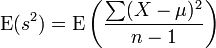
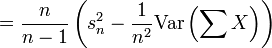
A common method is estimating the variance of large (finite or infinite) populations from a sample. We take a sample $(y_1,\dots,y_n)$ of n values from the population, and estimate the variance on the basis of this sample. There are several good estimators. Two of them are well known:

$s_n^2 = \frac 1n \sum_{i=1}^n \left(y_i - \overline{y} \right)^ 2 = \left(\frac{1}{n} \sum_{i=1}^{n}y_i^2\right) - \overline{y}^2,$

and

$s^2 = \frac{1}{n-1} \sum_{i=1}^n\left(y_i - \overline{y} \right)^ 2 = \frac{1}{n-1}\sum_{i=1}^n y_i^2 - \frac{n}{n-1} \overline{y}^2,$

Both are referred to as sample variance. Most advanced electronic calculators can calculate both s_n² and s² at the press of a button, in which case that button is usually labeled σ² or σ_n² for s_n² and σ_n-1² for s².

The two estimators only differ slightly as we see, and for larger values of the sample size n the difference is negligible. The second one is an unbiased estimator of the population variance, meaning that its expected value $E [s 2]$ is equal to the true variance of the sampled random variable. The first one may be seen as the variance of the sample considered as a population.

${}\operatorname{E}(s^2) = \operatorname{E}\left(\frac {\sum( X - \mu ) ^ 2}{n-1}\right)$

${}= \frac{1}{n-1} \operatorname{E}\left(\sum( X^2 -2X \mu + \mu^2)\right)$

${}= \frac{1}{n-1} \sum\left( \operatorname{E}(X^2) -\operatorname{E}(2X \mu) + \operatorname{E}(\mu^2)\right)$

${}= \frac{1}{n-1}\left( n\operatorname{E}(X^2) -2n\operatorname{E}(\mu^2) + n\operatorname{E}(\mu^2)\right)$

${}= \frac{n}{n-1}\left( s_n^2 + \mu^2 -\operatorname{E}(\mu^2)\right)$

${}= \frac{n}{n-1}\left( s_n^2 + \mu^2 -\operatorname{Var}(\mu)-\operatorname{E}(\mu)^2\right)$

${}= \frac{n}{n-1}\left( s_n^2 -\frac{1}{n^2}\operatorname{Var} \left(\sum X \right)\right)$

${}= \frac{n}{n-1}\left( s_n^2 -\frac{1}{n^2}ns_n^2\right)$

${}=s_n^2$

Common sense would suggest to apply the population formula to the sample as well. The reason that it is biased is that the sample mean is generally somewhat closer to the observations in the sample than the population mean is to these observations. This is so because the sample mean is by definition in the middle of the sample, while the population mean may even lie outside the sample. So the deviations to the sample mean will often be smaller than the deviations to the population mean, and so, if the same formula is applied to both, then this variance estimate will on average be somewhat smaller in the sample than in the population.

One common source of confusion is that the term sample variance may refer to either the unbiased estimator $σ 2$ of the population variance, or to the variance $s 2$ of the sample viewed as a finite population. Both can be used to estimate the true population variance. Apart from theoretical considerations, it doesn't really matter which one is used, as for small sample sizes both are inaccurate and for large values of n they are practically the same. Naively computing the variance by dividing by n instead of n-1 systematically underestimates the population variance. Moreover, in practical applications most people report the standard deviation rather than the sample variance, and the standard deviation that is obtained from the unbiased n-1 version of the sample variance has a slight negative bias (though for normally distributed samples a theoretically interesting but rarely used slight correction exists to eliminate this bias). Nevertheless, in applied statistics it is a convention to use the n-1 version if the variance or the standard deviation is computed from a sample.

In practice, for large $n$ , the distinction is often a minor one. In the course of statistical measurements, sample sizes so small as to warrant the use of the unbiased variance virtually never occur. In this context Press et al.^[3] commented that if the difference between n and n−1 ever matters to you, then you are probably up to no good anyway - e.g., trying to substantiate a questionable hypothesis with marginal data.

[edit] Distribution of the sample variance

Being a function of random variables, the sample variance is itself a random variable, and it is natural to study its distribution. In the case that $y i$ are independent observations from a normal distribution, Cochran's theorem shows that $s 2$ follows a scaled chi-square distribution:

$(n-1)\frac{s^2}{\sigma^2}\sim\chi^2_{n-1}.$

As a direct consequence, it follows that $\operatorname{E}(s^2)=\sigma^2.$

However, even in the absence of the Normal assumption, it is still possible to prove that $s 2$ is unbiased for $σ 2$ .

[edit] Generalizations

Unbiased estimate for expected error in the mean of A for a sample of M data points with sample bias coefficient ρ. The log-log slope -½ line for ρ=0 is the unbiased standard error.

If $X$ is a vector-valued random variable, with values in $\mathbb{R}^n$ , and thought of as a column vector, then the natural generalization of variance is $\operatorname{E}((X - \mu)(X - \mu)^\operatorname{T})$ , where $\mu = \operatorname{E}(X)$ and $X^\operatorname{T}$ is the transpose of $X$ , and so is a row vector. This variance is a positive semi-definite square matrix, commonly referred to as the covariance matrix.

If $X$ is a complex-valued random variable, with values in $\mathbb{C}$ , then its variance is $\operatorname{E}((X - \mu)(X - \mu)^*)$ , where $X *$ is the complex conjugate of $X$ . This variance is also a positive semi-definite square matrix.

If one's (real) random variables are defined on an n-dimensional continuum x, the cross-covariance of variables A[x] and B[x] as a function of n-dimensional vector displacement (or lag) Δx may be defined as σ_AB[Δx] ≡ 〈(A[x+Δx]-μ_A)(B[x]-μ_B)〉_x. Here the population (as distinct from sample) average over x is denoted by angle brackets 〈〉_x or the Greek letter μ.

This quantity, called a second-moment correlation measure because it's a generalization of the second-moment statistic variance, is sometimes put into dimensionless form by normalizing with the population standard deviations of A and B (e.g. σ_A≡Sqrt[σ_AA[0]]). This results in a correlation coefficient ρ_AB[Δx] ≡ σ_AB[Δx]/(σ_Aσ_B) that takes on values between plus and minus one. When A is the same as B, the foregoing expressions yield values for autocovariance, a quantity also known in scattering theory as the pair-correlation (or Patterson) function.

If one defines sample bias coefficient ρ as an average of the autocorrelation-coefficient ρ_AA[Δx] over all point pairs in a set of M sample points^[4], an unbiased estimate for expected error in the mean of A is the square root of: sample variance (taken as a population) times (1+(M-1)ρ)/((M-1)(1-ρ)). When ρ is much greater than 1/(M-1), this reduces to the square root of: sample variance (taken as a population) times ρ/(1-ρ). When |ρ| is much less than 1/(M-1) this yields the more familiar expression for standard error, namely the square root of: sample variance (taken as a population) over (M-1).

[edit] History

The term variance was first introduced by Ronald Fisher in his 1918 paper The Correlation Between Relatives on the Supposition of Mendelian Inheritance^[5]:

The great body of available statistics show us that the deviations of a human measurement from its mean follow very closely the Normal Law of Errors, and, therefore, that the variability may be uniformly measured by the standard deviation corresponding to the square root of the mean square error. When there are two independent causes of variability capable of producing in an otherwise uniform population distributions with standard deviations $θ 1$ and $θ 2$ , it is found that the distribution, when both causes act together, has a standard deviation $\sqrt{\theta_1^2 + \theta_2^2}$ . It is therefore desirable in analysing the causes of variability to deal with the square of the standard deviation as the measure of variability. We shall term this quantity the Variance...

[edit] Moment of inertia

The variance of a probability distribution is analogous to the moment of inertia in classical mechanics of a corresponding mass distribution along a line, with respect to rotation about its center of mass. It is because of this analogy that such things as the variance are called moments of probability distributions. The covariance matrix is related to the moment of inertia tensor for multivariate distributions. The moment of inertia of a cloud of n points with a covariance matrix of $Σ$ is given by

$I=n (\mathbf{1}_{3\times 3} \operatorname{tr}(\Sigma) - \Sigma).$

This difference between moment of inertia in physics and in statistics is clear for points that are gathered along a line. Suppose many points are close to the x and distributed along it. The covariance matrix might look like

$\Sigma=\begin{bmatrix}10 & 0 & 0\\0 & 0.1 & 0 \\ 0 & 0 & 0.1\end{bmatrix}.$

That is, there is the most variance in the x direction. However, physicists would consider this to have a low moment about the x axis so the moment-of-inertia tensor is

$I=n\begin{bmatrix}0.2 & 0 & 0\\0 & 10.1 & 0 \\ 0 & 0 & 10.1\end{bmatrix}.$

[edit] See also

Statistics portal

[edit] References

^ Michel Loeve, "Probability Theory", Graduate Texts in Mathematics, Volume 45, 4th edition, Springer-Verlaf, 1977, p. 12.
^ A. Kagan and L. A. Shepp, "Why the variance?", Statistics and Probability Letters, Volume 38, Number 4, 1998, pp. 329–333. (online [1])
^ Press, W. H., Teukolsky, S. A., Vetterling, W. T. & Flannery, B. P. (1986) Numerical recipes: The art of scientific computing. Cambridge: Cambridge University Press. (online)
^ P. Fraundorf (1980) "Microcharacterization of interplanetary dust collected in the earth's stratosphere" (Ph.D. Dissertation in Physics, Washington University, Saint Louis MO), Appendix E
^ Ronald Fisher (1918) The correlation between relatives on the supposition of Mendelian Inheritance

[edit] External links

[0] Michel Loeve, "Probability Theory", Graduate Texts in Mathematics, Volume 45, 4th edition, Springer-Verlaf, 1977, p. 12.

[1] A. Kagan and L. A. Shepp, "Why the variance?", Statistics and Probability Letters, Volume 38, Number 4, 1998, pp. 329–333. (online [1])

[2] Press, W. H., Teukolsky, S. A., Vetterling, W. T. & Flannery, B. P. (1986) Numerical recipes: The art of scientific computing. Cambridge: Cambridge University Press. (online)

[3] P. Fraundorf (1980) "Microcharacterization of interplanetary dust collected in the earth's stratosphere" (Ph.D. Dissertation in Physics, Washington University, Saint Louis MO), Appendix E

[4] Ronald Fisher (1918) The correlation between relatives on the supposition of Mendelian Inheritance

[1]

[2]

[3]

[4]

[5]