łŘ˝ŃľđĘó˝čÍý¸¦µć No.1 1997 pp.25-34
New Data Compression for Multi-Dimensional Numerical Simulation
Mitsue Den , Kazuyuki Yamashita *,
Ryoji Matsumoto **
Hiraiso Solar Terrestrial Research Center, Communications Research Laboratory,
3601 Isozaki, Hitachinaka, Ibaraki 311-12
TEL: 029-265-9729ˇˇFAX: 029-265-9728ˇˇden@crl.go.jp
*Information Processing Center, Chiba University,
1-33 Yayoi, Inage, Chiba 263
TEL: 043-290-3536ˇˇFAX: 043-290-3544ˇˇyamasita@ipc.chiba-u.ac.jp
**Department of Physics, Faculty of Science,
Chiba University,
1-33 Yayoi, Inage, Chiba 263
TEL: 043-290-3724ˇˇFAX: 043-290-3720ˇˇmatumoto@c.chiba-u.ac.jp
Abstract
ˇˇWe present a new data compression algorithm, useful for a visualization
and a rough analysis of multi-dimensional numerical simulation results with
mesh code. The algorithm consists of a classification or a quantization of
single or double precision real data at each mesh point, and a subsequent
compression by using a conventional compression algorithm. We describe a
data compression method in detail, showing this method does work for
several typical problems existing in the numerical simulation in
astrophysics by counting a compression efficiency. We also investigate a
relation of the compression efficiency and simplicity or complexity of the
data distribution. When single precision real data on mesh points are
compressed by using 8-bit quantization, the compression rate is at least
75% for complex distribution and more than 93% for simple distribution. A
source program based on our compression algorithm written in FORTRAN
language is now available for interests.
Keywords
Data compression, Image processing, Information processing, Numerical methods
1 Introduction
ˇˇNumerical simulation recently becomes a powerful tool in the natural
sciences. With an increase of a processing speed of super computers,
we can perform
multi-dimensional numerical simulations, yielding a real world in the
computer. We are, however, facing problems to have to handle a huge amount
of data at the same time when they perform multi-dimensional simulations.
Furthermore, we must save data at some interval to obtain results with high
resolution in time. The interval, however, is limited by a disk space for a
storage and a speed in handling data. The super computer is also used by many
users, sharing the disk space and cpu time. Each user has a finite disk
space and a finite cpu time, so important simulation results may be missed
due to the limited number of snapshots available.
ˇˇTo overcome this dilemma, we will propose a new compression algorithm. Data
compression is a very powerful way to resolve the above mentioned problems,
since it can reduce a data volume. Users can frequently write their dynamical
simulation results to files and can save cpu time for the output, also.
ˇˇData compression method has been proposed by many authors. It can be
divided into two groups; i.e. 'lossless' and 'lossy' methods. Lossless means
that the compressed data can be restored perfectly. An example is a gzip
which mainly operates in a unix machine. The method is appropriate for the
sequential and not so large text data. On the other hand, lossy compression
method can archive drastic compression, because it loses lots of information
from the original data literally. The compression algorithm is apposite to
the image data. The lossy method has a common risk: i.e. failure of a
compression. The meaning of 'failure' or 'success' is as follows. If an
image drawn with compressed data bears comparison with an image drawn with
the original data, it is successful. There is a case when an apparent
difference exists between an image drawn by compressed data and original
image. This case fails in compression. Typical lossy compression method is
JPEG. This method depends on the data and a compression is not always
successful.
ˇˇIt should be noted that there is a case in which compression fails by
lossless method, where a 'failure' has different meaning from the word used
in lossy methods: i.e. the failure case is that the volume of compressed
file is comparable with or even larger than that of the original file. So,
the compression is, generally, very useful but its success depends on the
original data.
ˇˇIn this paper, we introduce a new algorithm of a data compression. The data
which we target are like image data, which are mainly used for visualization
and the volume is huge. Since the data require drastic compression, our
compression algorithm can be lossy rather than lossless. On the other hand,
numerical data obtained by the numerical simulations can be sequential stream
of characters (text) like the data usually compressed by lossless methods.
Our compression method, therefore, can be placed in the medium between above
two groups.
ˇˇIn the next section, we describe the algorithm of the compression, show the
compression efficiency obtained in the astrophysical models, and compare the
contour maps of time evolution of numerical simulation. A galaxy formation
will be drawn with the compressed data by our algorithm and with the original
data. Summary and future work will be given in Section 3.
2 Data Compression Method and Compression Efficiency
ˇˇAn aim is to find a compression algorithm to select necessary and enough
information for graphical representation of the results of multi-dimensional
numerical simulation with mesh code. Many authors draw contour maps to find
some physical meanings in simulation data. We, therefore, set the criterion
of 'success' of compression: if the contour maps drawn with the compressed
data, we call compressed map in the following, are comparable with those
with the original data, called the original map, the compression is
successful. The word 'comparable' may be still ambiguous. In other word, if
we can find the same physics in the compressed map as can be seen in the
original map, we say that the compressed map is comparable with the original
map.
ˇˇThe key point is a way to abstract minimal and necessary information from
the original data. Our compression algorithm is as follows.
- Set contour levels enough for covering a dynamic range of original data.
- Classify the original data according to the specified contour levels.
- Make a table of relation between the data and the contour levels.
Data belonging to the same contour level are regarded as the same value.
Information is lost here and then the data are compressed.
ˇˇIf the data distribute linearly with one peak, the following simplest
process can be applied:
- Find the minimum and maximum value of the original data.
- Divide the range between the minimum and the maximum equally into the
number of the contour levels, say, 1byte=256.
- Convert the original data value at each grid point into the number of
corresponding contour level (Classification).
- Make a conversion table which records the original level corresponding
to each number of contour level.
If the dynamic range of the original data is very large, the logarithm of
those data is calculated and then classified into the contour level.
ˇˇThis method is also applicable to the more complicated cases such as that
the density distribution has two peaks or to the vector fields such as
velocities or magnetic field. We return to this point in the final section.
As for the number of levels, we can use more than 256 levels, if necessary.
The file size of table is given by (4byte ˇß number of contour level
+ header of file ˇÁ 1Kbyte). If the original data are expressed in
single precision, those volume are compressed to about a quarter in this part
of our algorithm.
ˇˇSince the compressed data are still sequential text (i.e., stream of
characters), we can compress them furthermore by using lossless compress tool.
Thus, in our algorithm, the data go through compression twice. As the
lossless compression tool in the second part, we adopt the LZW15V.C in this
paper. The algorithm of this tool is based on LZW and it is same as
'compress' which is very familiar for unix machine users (see reference). The
source program of the first compression tool based on our algorithm is
written in FORTRAN language and that of the second one is written in C
language which is public, so we can compress the data in the application
program from which the compression programs described above are called. We
release those subroutines to public such that anyone who wants can use them
(please contact the first author). It is noted that any lossless compression
tools are available for the second compression tool.
ˇˇThe compression efficiency (CE) is defined by

where m is the volume of the compressed data, called map data and
r is the volume of the original data, called raw data. This definition
means that as CE tends to 1, compression is more efficient. If CE is
negative, which case is possible in general, that compression is in failure.
Since the size of the map data is always a quarter of the the original data
based on our compression algorithm when the raw data are expressed in single
precision, the compression efficiency is always 75% for this part.
ˇˇFirst, we obtain CE for the snapshot data of the density with one peak for
three models which are
- Parker solution of solar wind as a model of simplex structure in which density varies linearly.
- Cluster of galaxies which are simulated hydrodynamically as a model of several clumps whose densities also vary linearly.
- Expanding supernova ejecta as the model of a logarithmic density distribution.
For model I, the data are obtained by one-dimensional numerical simulation in
spherical coordinate and is converted to 3D data in Cartesian coordinate. For
models II and III, they are snapshots of time evolution followed by
three-dimensional numerical simulation in Cartesian coordinate.

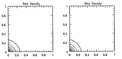
Fig.1 Contour maps of the density drawn with the raw data and with the map data
for Model I. Two-dimensional plot on z=constant surface.

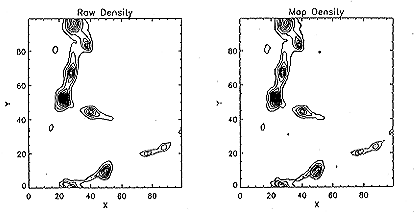
Fig.2 Same maps as figure 1 but for Model II.

Fig.3 Same maps as figure 1 but for Model III
ˇˇThe contour map of the density drawn with the raw data and with the map
data for Models I, II and III are shown in figures 1, 2 and 3, respectively.
There are some differences between two pictures in the low density region in
figure 3. However, the main structure; i.e. the high density region, can be
reproduced by the map data in this model. It is noted that the interesting
physical process does not always proceed in the high density region when the
system includes magnetic field. In that case, the analysis using only the
density contour maps is not enough and the maps of the magnetic fields and/or
velocities are also needed. We will investigate this in the next paper. At
least we can say that the compressed map is comparable with the original map
in model III and that these compression can be regard as successful for three
models.

ˇˇIn table 1, we show the volume of the raw data(R), the volume of the map
data(M), the volume of twice compressed data(C2) of the map data. The
compression efficiency is larger than 93% for each model. The original data
can be decreased to be less than %, 1.9% for model II which shows the most
complicate plot and has the largest volume of the data.
ˇˇThis is very important because we can store data of ten times larger (about
fifty times for model II ) time steps for the analysis of time evolution
under the same disk space condition. This means the time evolution of our
interesting phenomena can be traced in detail, so it is possible for us to
find physics which may be missed in the coarse snapshots. The cpu time is
also limited in most super computer systems. If the cpu time for I/O cannot
be negligible in one job class, reducing the volume of output data enables
us to increase cpu time for processing operation under the constant number
of snapshots. In order to investigate this point, we follow the time
evolution of galaxy formation by 3D numerical simulation. In this
calculation, we insert the subroutines for the compression and write the
compressed data as well as the raw data for comparison to files. We save the 50 mapdata snapshots and the 4 raw data snapshots.

ˇˇThe CPU time is given in table 2. The ratio of the CPU time including
execution of compression and output of the data to the total CPU time is
about 1.7%. We can say that it is negligible. The cpu time for execution of
compression at one time is 0.67 sec, that for execution of the second
lossless compression and for I/O of the map data at one time is 4.33 sec and
that for I/O of the raw data at one time is 3.25 sec. The cpu time for only
I/O of the map data cannot be compared with that of the raw data, because it
is difficult to abstract the cpu time for I/O from 4.33 sec. However, the
volume of the map data is always less than a quarter of the volume of the raw
data, then we expect tio-map < tio-raw.
So the cpu time for execution
and I/O of compression is negligible.

ˇˇThe file sizes of the raw data and the compression efficiencies of selected
map data from 50 snapshots are shown in table 3. The file size of the raw
data is same for all four snapshot data. The CE is nearly 75% at the initial
time, which means the second lossless compression almost does not work
because the CE of the second compression tool may be related to simplicity
of the configuration of distribution of the data, and there are no simple
structures initially in this simulation model. This model is same as Model
II. The configuration of the density distribution and CE are different from
those of Model II (see figure 2 and figures 4a, 4b in the following) because
we calculate the logarithm of the data and then classify those data into the
contour level in this calculation. Since degeneracy of the contour of the
density is relaxed, more complicated structure appears and CE becomes low.
We take 251 contour levels, so the file size of the table is negligible
compared with the total file size of the map data.


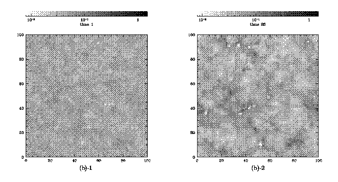
Fig.4 Density maps in a shade of monochromatic color on z=constant surface.
The raw data 4a-A ˇÁ 4a-Z and selected map data 4b-1 ˇÁ 4b-50 are lined in time
sequence.
ˇˇWe present the density maps in a shade of monochromatic color in figures 4a
and 4b which demonstrate time evolution by the raw data(4a) and by selected
map data(4b). The figures 4a-A and 4b-1 are snapshots at the same time and
the figures 4a-C and 4b-50 are also snapshots at the same time (there are no
corresponding figures for 4a-B and 4a-Z in figures 4b and figure 4b-Z shows
later stage than figure 4a-C or 4b-50). These plots show the process of
galaxy formation. At the initial time (figures 4a-A or 4b-1) there are not so
large depth in the shade since the gas distributes without any structures. As
time evolves, the gas gathers and makes high density region (drawn in black
color) owing to gravitational instability and the large scale structures
appear as seen in the final map (figures 4a-Z or 4b-50). We can see little
differences in these pairs and again compression is successful for this
model. The CE almost grows monotonously according to time evolution as shown
in figure 5 because the configuration is simplified after formation of the
large scale structure. It is suggested that the CE may be a kind of index of
complexity of configuration like entropy in hydrodynamics or genus count in
geometry.

Fig.5 Time evolution of compression efficiency. The horizontal axis is
a scale of the univers,
which plays a role of time because it grows
monotonously.
ˇˇFurthermore, since the volume of the map data is small, handling of those
data is speedy and light. For example, the maps in figures 4a and 4b are
drawn on two-dimensional surface at z=constant. We can see the maps at
other surface easily by using the map data. We conclude that the map data is
very useful for analyzing the numerical data.
3 Summary
ˇˇWe have introduced a new compression algorithm for multi-dimensional
numerical simulation results with mesh code. The compression efficiency is
always more than 75% if the original data are expressed in single precision.
Our compression method is, therefore, apposite to huge amount of data like
the images and is useful for visualization or rough analysis of numerical
results.
ˇˇSince the compressed data by our method is still sequential text, we can
compress those data once more by lossless method. We adopt LZW15V.C whose
source code is public. We wrote the subroutine program in FORTRAN language
for our compression method for the propose that any one can use the
subroutines of our method and LZW15V.C written in C language.
ˇˇWe have shown the practical applicability of this method by adopting three
typical models. The final CE are more than 93% for three models. Those CEs
depend on the second lossless compression tool and may depend on the
configuration of the data distribution. In order to investigate this
point, we
simulated time evolution of galaxy formation numerically and wrote the map
data at 50 times and the raw data at 4 times to files. The cpu time necessary
for compression is negligible, compared with the total cpu time and the CE
grows up as the configuration becomes simplified. Thus we suggest that the
CE may be regard as a kind of indices showing simplicity or complexity.
ˇˇWe adopted the simplest setting for the contour level and applied this only
to the density variable in this paper. However, some device is needed e.g.
for the case that the distribution has two peaks or for the vector variables.
The contour level is not necessarily be set equally and it is better that it
is set automatically with constant degree of information loss according to
change of minimum and maximum of data and of distribution. In the next paper,
we will present the improved compression tool and will apply the renewed tool
to the vector variables.
ˇˇThis method also can be used for volume data in AVS which is one of
graphical software and many people use for multi-dimensional graphics. The
visualization is very important for analysis of multi-dimensional numerical
simulation data, so in future we will present the I/O module for AVS and/or
IDL (also the graphical software) which will be welcomed by researchers who
work with numerical simulation.
Acknowledgment
ˇˇWe would like to thank Dr. T. Obara for careful reading of this manuscript.
References
- [1]
- Nelson M., Gailly J.-L. 1996, in The Data Compression Book, Second Edition, (Prentice Hall, Toppan, Tokyo) p245
(Received 25 July 1997 ; accepted 15 August 1997)
ˇĘ1997ÇŻ7·î25ĆüĽőÍýˇ¨1997ÇŻ8·î15ĆüşÎĎżˇË


